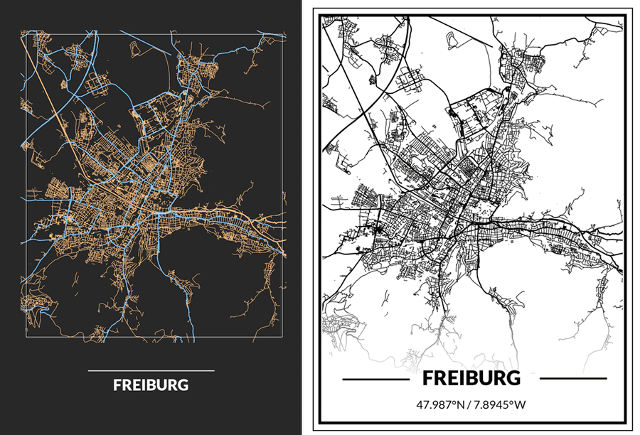
A popular gift among friends is a streetmap. The streetmap is meant to be a reminder of good times and to accompany a person when they have long since moved out of a city. Such streemaps can be bought on the internet. But we don't have to spend so much money on streetmaps because we can achieve similar results with ggplot2.
In this tutorial, you'll learn how to create streetmaps for any city. We will use the packages osmdata and ggplot2. With osmdata we can extract the streets from the Openstreetmap database. Openstreetmap is a freely available database of all locations in the world under an open license. Therefore, we don't need an API key or the like to get the data. As always, tidyverse is our tool to create visualizations and wrangle the data.
Since I haven't worked very much with maps in ggplot2 yet, I had to find some good blogposts online first. Many thanks especially to Dominic Royé for his detailed blog article which I used as an orientation for this tutorial.
Since I myself currently live in the city of Freiburg in the south of Germany, we will create the tutorial using this city. However, you can take any other city. All you have to do later is adjust the longitude and latitude of your city. Here you can see the two results we will create at the end of this tutorial:
First, as always we have to load the necessary packages:
library(tidyverse)
library(osmdata)
Before we start working with R we must understand how OpenStreetMap stores streets. Check out this web page for a full reference. OpenStreetMap describes all physical things (e.g. a house) as features. These features are stored as key value pairs. For example, there is a key called highway. A highway can be an ordinary street. For example, there are highways that lead to residential buildings (residential). Other highways connect larger cities with each other (primary). To get all tags of a feature via osmdata, you can enter the following function:
available_tags("highway")[1] "bridleway" "bus guideway" "bus stop" "construction"
[5] "crossing" "cycleway" "elevator" "emergency access point"
[9] "escape" "footway" "give way" "living street"
[13] "milestone" "mini roundabout" "motorway" "motorway junction"
[17] "motorway link" "passing place" "path" "pedestrian"
[21] "platform" "primary" "primary link" "proposed"
[25] "raceway" "residential" "rest area" "road"
[29] "secondary" "secondary link" "service" "services"
[33] "speed camera" "steps" "stop" "street lamp"
[37] "tertiary" "tertiary link" "toll gantry" "track"
[41] "traffic mirror" "traffic signals" "trailhead" "trunk"
[45] "trunk link" "turning circle" "turning loop" "unclassified" The output shows you all types of streets that OpenStreetMap saves. You can display a list of all features with the following command:
available_features()I'm not going to show you the whole list now because it's pretty long. Now that we know which tags are under the highway feature, we can start exporting the data from the database. But for this we should first know were our city exactly is in the world. A handy function to do this is get_bb from the osmdata package. To get the cooordinates of our city we need to add the city and the country of the city as a string. Freiburg im Breisgau for example in southern Germany can be found as follows:
getbb("Freiburg im Breisgau Germany") min max
x 7.662006 7.930844
y 47.903578 48.071058This now gives us the coordinates of the city. The x-value indicates the longitude of the city, the y-values the latitude. More information about this system can be found here. For example, a positive latitude indicates that Freiburg is north of the equator. Auckland in New Zealand has a negative latitude because New Zealand is south of the equator:
getbb("Auckland New Zealand") min max
x 174.6032 174.9232
y -37.0121 -36.6921Now that we know the coordinates, we can export the roads from the coordinate system. To do this, we must first pass the output of the getbb function to the opq function. To be honest, I'm not so sure what the function does, but we need it. Next, we transfer this output to the function add_osm_feature. The function has two arguments. With key we specify the key of the feature, with value we specify the tag of the feature. In our case, we first extract all major streets of the city of Freiburg from the dataset. Finally we transfer the output into the function osmdata_sf to insert it later into ggplot2.
streets <- getbb("Freiburg Germany")%>%
  opq()%>%
  add_osm_feature(key = "highway",
                  value = c("motorway", "primary",
                            "secondary", "tertiary")) %>%
  osmdata_sf()
streets
Object of class 'osmdata' with:
$bbox : 47.9035777,7.6620055,48.0710579,7.9308444
$overpass_call : The call submitted to the overpass API
$meta : metadata including timestamp and version numbers
$osm_points : 'sf' Simple Features Collection with 15294 points
$osm_lines : 'sf' Simple Features Collection with 4079 linestrings
$osm_polygons : 'sf' Simple Features Collection with 7 polygons
$osm_multilines : NULL
$osm_multipolygons : NULLThe data from the database is now stored in the streets variable. This object has different child objects. Later osm_lines are especially interesting for us. osm_points are more interesting for places. The function add_osm_feature is much more powerful than described here. If you want to learn more about it, see the official documentation of the package. There you'll find, for example, how to nest several questions together. For example, where are all the Irish pubs in a city?
Next we get the smaller streets and the main river of Freiburg (the Dreisam) from the database:
small_streets <- getbb("Freiburg im Breisgau Germany")%>%
  opq()%>%
  add_osm_feature(key = "highway",
                  value = c("residential", "living_street",
                            "unclassified",
                            "service", "footway")) %>%
  osmdata_sf()

river <- getbb("Freiburg im Breisgau Germany")%>%
  opq()%>%
  add_osm_feature(key = "waterway", value = "river") %>%
  osmdata_sf()
Let's create our first streetmap:
ggplot() +
  geom_sf(data = streets$osm_lines,
          inherit.aes = FALSE,
          color = "black",
          size = .4,
          alpha = .8) +
  coord_sf(xlim = c(7.77, 7.92),
           ylim = c(47.94, 48.06),
expand = FALSE) 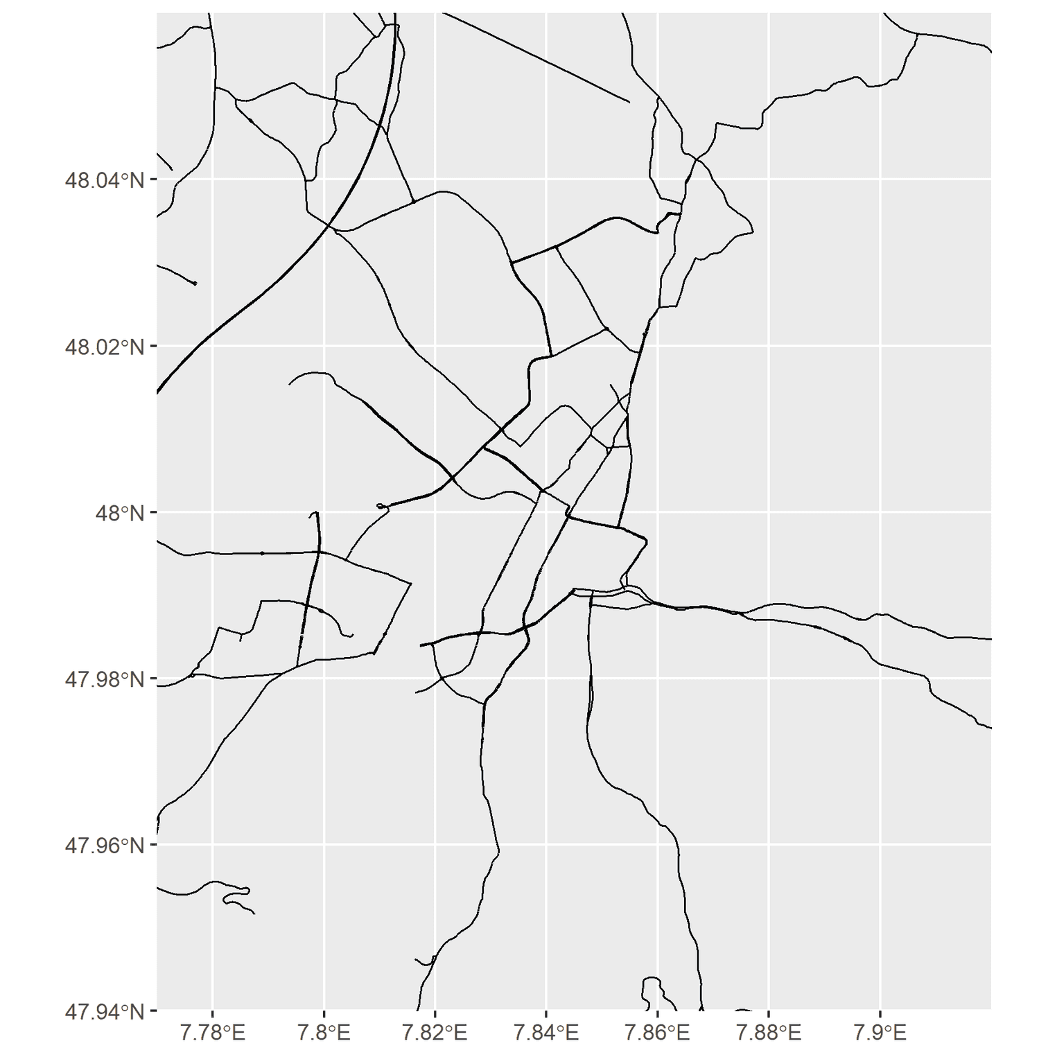
First, we add the geom geom_sf to the function ggplot. For data we add the streets stored in the variable streets$osm_lines. We can determine the width of the streets with size. At the same time I don't want to make the streets totally black, so I make them a bit transparent by changing the alpha level. With the function coord_sf I can determine the x- and y-axis exactly. It is best to play around with the values until you have defined the right limits for yourself. With expand = FALSE you make sure that the coordinates are displayed exactly.
Next, let's add the small streets and our river:
ggplot() +
  geom_sf(data = streets$osm_lines,
          inherit.aes = FALSE,
          color = "black",
          size = .4,
          alpha = .8) +
geom_sf(data = small_streets$osm_lines, inherit.aes = FALSE, color = "black", size = .4, alpha = .6) + geom_sf(data = river$osm_lines, inherit.aes = FALSE, color = "black", size = .2, alpha = .5) + coord_sf(xlim = c(7.77, 7.92), ylim = c(47.94, 48.06), expand = FALSE) 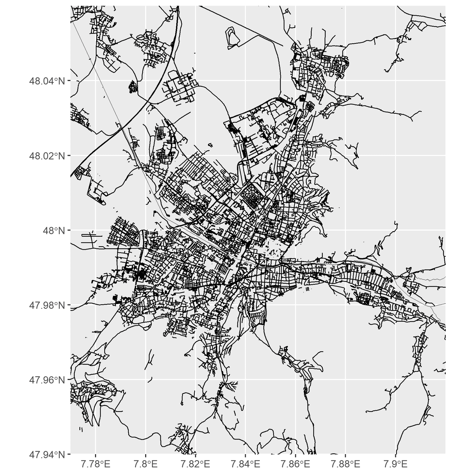
You can also highlight the streets in color if you want:
ggplot() +
  geom_sf(data = streets$osm_lines,
          inherit.aes = FALSE,
          color = "steelblue",          size = .4,
          alpha = .8) +
  geom_sf(data = small_streets$osm_lines,
          inherit.aes = FALSE,
          color = "black",
          size = .4,
          alpha = .6) +
  geom_sf(data = river$osm_lines,
          inherit.aes = FALSE,
          color = "black",
          size = .2,
          alpha = .5) +
  coord_sf(xlim = c(7.77, 7.92),
           ylim = c(47.94, 48.06),
expand = FALSE) 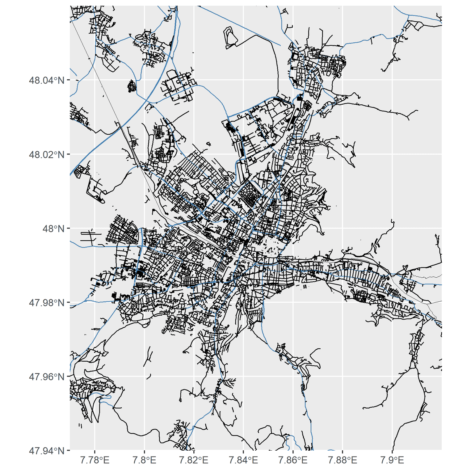
There's one more thing that's disturbing, though. The x- and y-axis. To remove them we can add the function theme_void():
ggplot() +
  geom_sf(data = streets$osm_lines,
          inherit.aes = FALSE,
          color = "steelblue",
          size = .4,
          alpha = .8) +
  geom_sf(data = small_streets$osm_lines,
          inherit.aes = FALSE,
          color = "black",
          size = .4,
          alpha = .6) +
  geom_sf(data = river$osm_lines,
          inherit.aes = FALSE,
          color = "black",
          size = .2,
          alpha = .5) +
  coord_sf(xlim = c(7.77, 7.92),
           ylim = c(47.94, 48.06),
           expand = FALSE) +
  theme_void()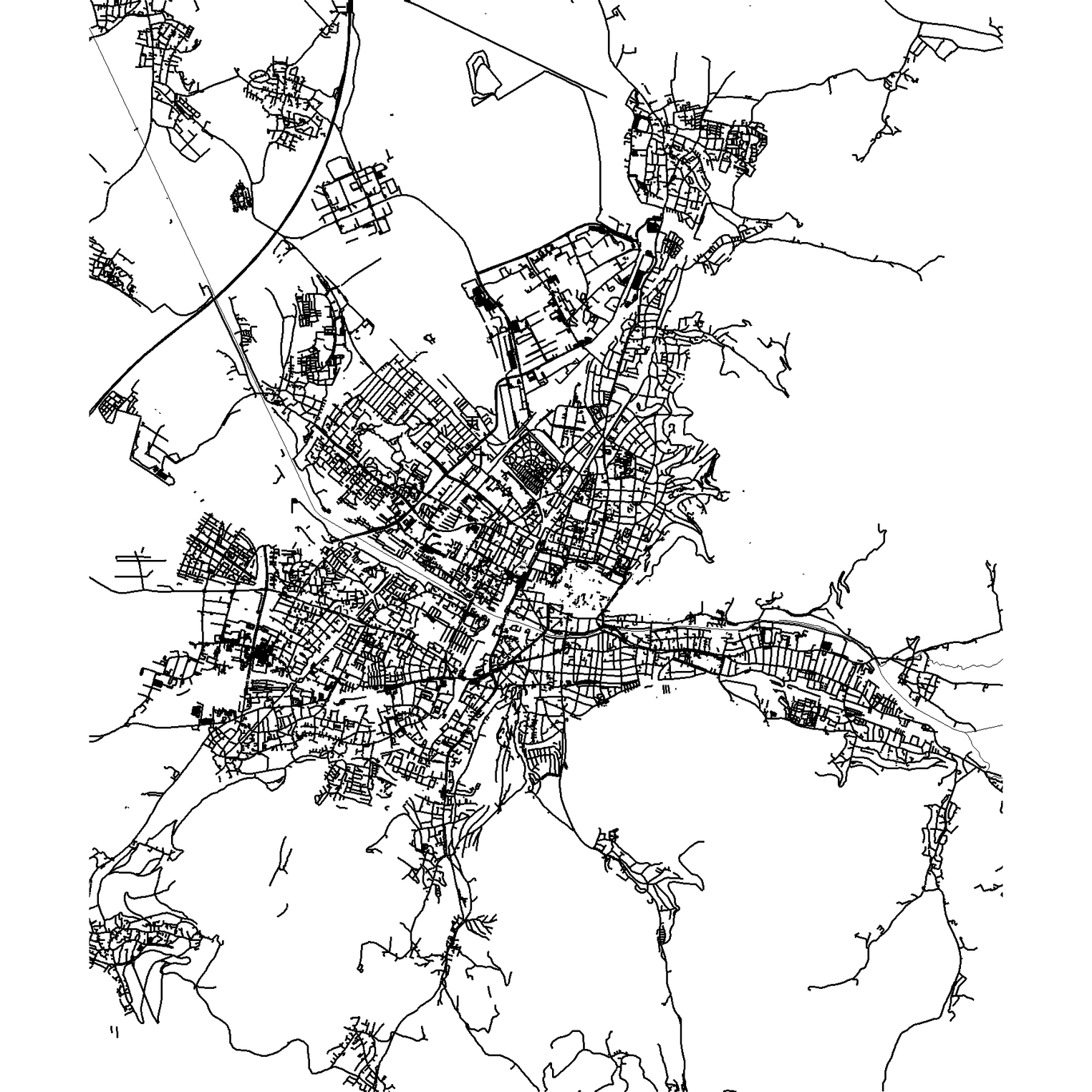
Next, we can adjust the colors of the visualization. I want to create not only a white streetmap, but also one with a dark background:
ggplot() +
  geom_sf(data = streets$osm_lines,
          inherit.aes = FALSE,
          color = "#7fc0ff",          size = .4,
          alpha = .8) +
  geom_sf(data = small_streets$osm_lines,
          inherit.aes = FALSE,
          color = "#ffbe7f",          size = .2,
          alpha = .6) +
  geom_sf(data = river$osm_lines,
          inherit.aes = FALSE,
          color = "#ffbe7f",          size = .2,
          alpha = .5) +
  coord_sf(xlim = c(7.77, 7.92),
           ylim = c(47.94, 48.06),
           expand = FALSE) +
  theme_void() +
  theme(    plot.background = element_rect(fill = "#282828")  )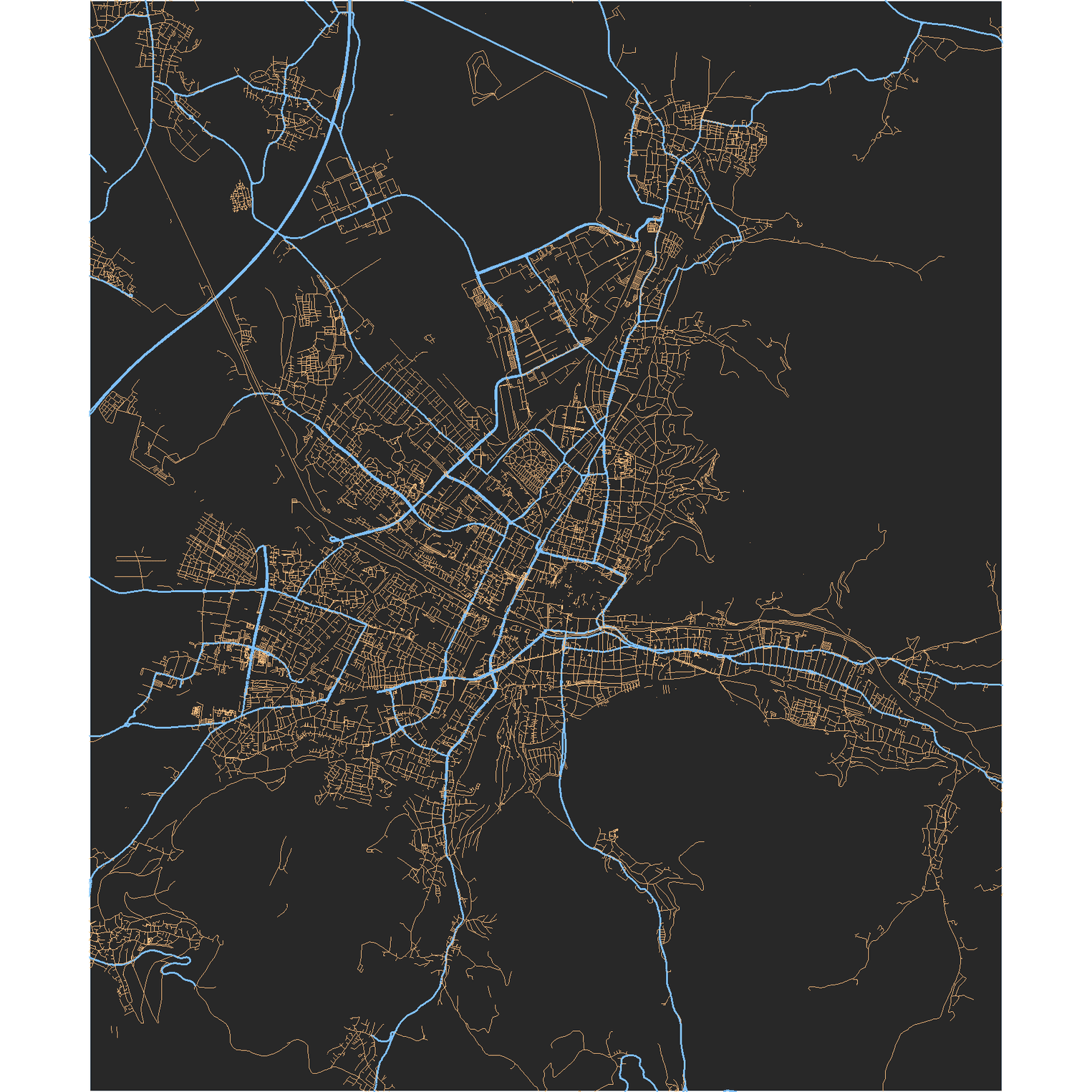
Now that we've created both visualizations, we can make a poster out of it. To do so I first exported the visualizations as a png file. Make sure that you execute the function right after you have created your streetmap.
ggsave("map.png", width = 6, height = 6)Next, I created a Powerpoint file and resized it. Then I imported the png file and enlarged it. You might also need to crop the png first. As text I used the font Lato. I recommend that you search the internet for photos of streetmaps and use these examples as a guide. There are already countless beautiful designs that you can recreate relatively easily in Powerpoint.
The examples from this tutorial can be found here. Feel free to share your own streetmaps on Twitter, I'm curious what you create.

